A simple framework for performance metrics
Select the best metric for your problem with ease
By Martin Helm in Data Science ML Classification Metrics MLOps
March 3, 2021
Accuracy, sensitivity, specificity, F1 score, … — the list of performance metrics is seemingly never-ending. Especially if you are new to data science, you can easily feel stranded in an ocean of choices. In this post I want to give you an introduction into a framework to group performance metrics, how they connect to each other and how you can use it to choose the best metric for your problem and model. The performance metric framework
You will surely have heard about metrics, such as accuracy, sensitivity, F1 score, receiver operating characteristic (ROC) and many more. But when I started to dive into them, I often asked myself, how they all relate to each other. After a while, I stumbled over a fantastic framework proposed by Ferri and colleagues that made things much easier for me.
Basically, we can group the common performance metrics for binary classification tasks into three categories. Each one of them serves a different purpose:
- Threshold metrics: Check whether your model satisfies a predefined threshold.
- Ranking metrics: Compare model instances or complete models against each other.
- Probability metrics: Measure the uncertainty of your classifications.
Let’s look at each one in order:
Threshold metrics
These are your day-to-day metrics, such as accuracy, F1, FDR, basically everything that it listed on this Wikipedia page. What they have in common is that you specify in advance which performance metric(s) matter to your given problem and define a threshold that your model needs to pass. And that is already where the name comes from. If your model does not pass your threshold, it will not even be considered further.
Threshold metrics are applicable to basically all classifier algorithms out there, independent whether they directly output a class label (like simple k-means or decision trees) or a class membership score (like fuzzy c-means or logistic regression).
I will not go into detail on how each of these metrics is calculated, that is beyond the scope of this article. If you are interested to learn about the individual metrics, check the references, where I listed some excellent sources.
What I do want to mention though is that it is especially important to check up front if you have a balanced or an imbalanced dataset. For imbalanced datasets, common metrics such as accuracy are already not suitable anymore, as a naive classifier always predicting the majority class will already have high accuracy. Instead, use metrics that focus on the minority class, which is the positive class by convention.
Ranking metrics
Ranking metrics are particularly useful when dealing with classifiers that output a class membership score. To transform this score into a crisp class label, you will need to apply a threshold to the score. But how to select this threshold? Ranking metrics make it a breeze. Let’s first assume you have a balanced dataset:
After training the model, iterate over all possible thresholds and calculate the True Positive Rate and the False Positive Rate. Then plot these against each other. You will end up with the so-called receiver operating characteristic, short ROC:

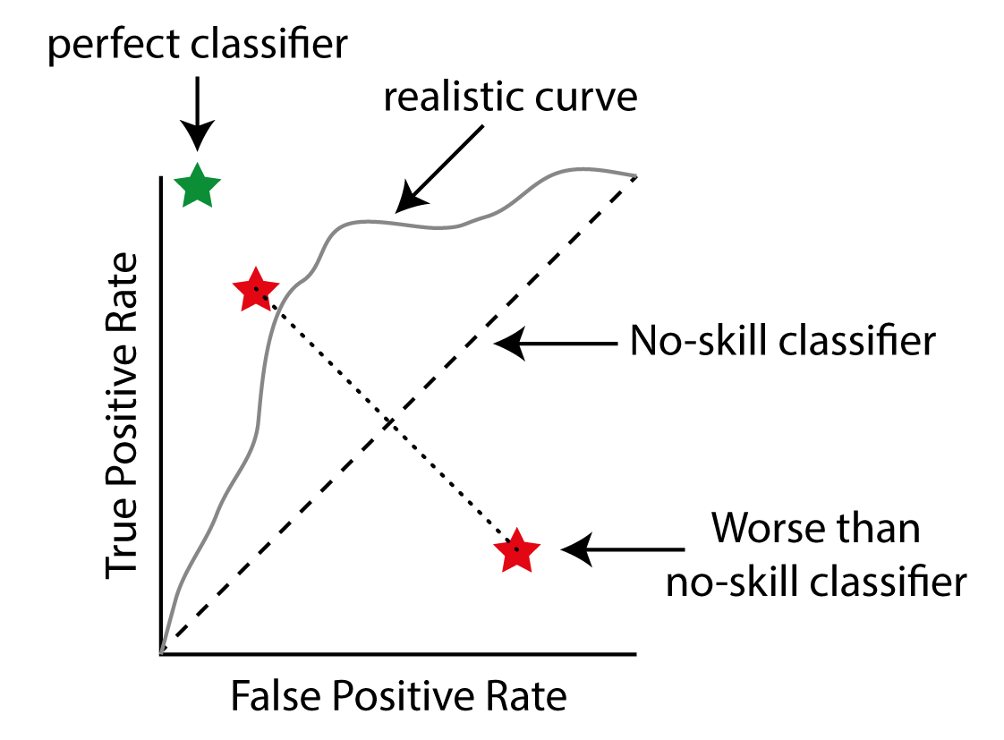
A schematic reciever operating characteristic. A perfect classifier will have a TPR of 1 and a FPR of 0, ending up in the top left corner (green star). A no-skill classifier finds as many True Positives as False Positives, indicated by the dashed line. By iterating over different thresholds for your model you can generate a curve depicting the behaviour of your model (grey line). A classifier that is worse than random can be converted into a skillfull classifier by simply selecting the opposite.
A perfect classifier will have a TPR of 1 and a FPR of 0, ending up in the top left corner (green star). A no-skill classifier finds as many True Positives as False Positives, indicated by the dashed line. By iterating over different thresholds for your model you can generate a curve depicting the behavior of your model (grey line). A classifier that is worse than random can be converted into a skillful classifier by simply selecting the opposite of its output. This will reflect its behavior along the diagonal (red stars). Image by the author.
A perfect classifier will be in the top left spot of this diagram. The diagonal depicts a naive classifier with no skill. You can think of it as a classifier that simply outputs random numbers, or always a fixed number. When you move the threshold, you will get more and more True Positives by chance, but at the same time your False Positives will equally increase. To select the best model, simply choose the point that is closest to the top left corner. You can easily do that by calculating True Positive Rate — False Positive Rate (which is also called Youden’s J statistic).
One interesting fact is, that models below the diagonal are not necessarily worse than random. By simply inverting whatever the model outputs, you can basically reflect its point by the diagonal and potentially gain a very skillful model.
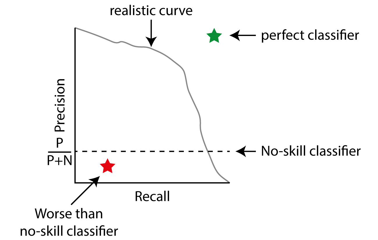
For imbalanced dataset, the corresponding plot is the Precision-Recall Curve. This time, the optimal classifier is at the top right (in contrast to ROC, where it is at the top left), and the naive classifier will produce a horizontal line that crosses precision (defined as TP/ (TP + FP)) at the fraction of positives in the dataset. This is because a no-skill classifier with random predictions has a chance equal to the fraction of real positives in the dataset to also predict it as a positive (negatives are note considered in precision!). At the same time, by moving the threshold, the no-skill classifier will correctly identify more and more positives, thus increasing the recall (defined as True Positives out of all positives).

A Precision-Recall curve for imbalanced datasets. The perfect classifier is now at the top right (green star), whereas a no-skill classifier always has constant precision. Iterating over the thresholds for your model will yield a behavior similar to the grey line.
To select the best threshold, calculate Precision + Recall and select the threshold of this spot (which is equal to selecting the model with the highest F1 score).
Probability metrics
Probability metrics are a bit special, because here we do not only deal with assessing whether our model did the right classification but are more interested in how certain it was for its classifications. As with ranking metrics, these can of course only be applied to models that output a class membership probability (which might need to be normalized before assessing them).
Using probability metrics, we can specifically penalize the model for making wrong classifications with high confidence, whereas errors where the model output was not very conclusive do not suffer such high cost. Note that an indecisive model in general will also not perform well in probability metrics, as they do reward strong and correct predictions as well.
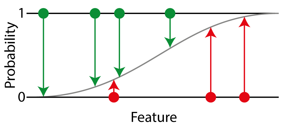
The most common probability metric is log-loss, also known as cross-entropy. Since it weights positives and negatives equally, you should only apply it to balanced datasets. Imagine a binary classification problem, to which we fit a logistic regression:

Visual explanation of log-loss. Imagine a one-dimensional problem, where each point simply is a number (x-axis). For each point, we know the true probability of being in the positive class, 1 for positives (green points) or 0 for negatives (red points). We fit a logistic regression to our problem to classify the points (grey line). The difference between the predicted probability to the true probability is then used to calculate the log-loss.
From our test set, we know the true probability of a given point to be in the positive class, which is 0 for negatives and 1 for positives. Our logistic regression assigns a probability that is in the range of 0 to 1. The log-loss is then based on the difference of our assigned probability to the true probability. For each point we calculate the log loss and average over all points.
$$ L_{log}(y, \hat y) = -1 {1 \over N} \sum_{i=1}^N {x * log(\hat y_i) + (1-y) * log(1-\hat y_i)} $$
For imbalanced datasets, you should again use a metric that is more focused on the positive class, for example the Brier score. It is defined as the Mean Squared Error between the expected and the predicted probability for the positive class:
$$ Brier Score = {1 \over N} \sum_{i=1}^N{\hat y_i - y_i)^2} $$
I hope this framework is as useful to you, as it was to me. First, decide on the threshold metric(s) most relevant to your project, then train you model and rank them with the ranking metrics. Finally, if you have probabilistic models, consider using probability metrics.
Of course, one of the difficult parts is still to decide which metric makes the most sense. For this the best way is usually to have an in-depth discussion with the domain experts what kind of error they really want to avoid. Or stay tuned for more to come on this problem as well.
References
Ferri, Hernandez-Orallo & Modroiu (2009): An experimental comparison of performance measures for classification. Pattern Recognition Letters
Photo by Clark Van Der Beken on Unsplash
- Posted on:
- March 3, 2021
- Length:
- 8 minute read, 1523 words
- Categories:
- Data Science ML Classification Metrics MLOps