A deep dive into partitioning around medoids

The final evolution of k-means and why you probably learned it wrong before

By Martin Helm in Data Science Machine Learning kmeans R pam

August 20, 2021

library(ggplot2)
library(gridExtra)
library(knitr)

Introduction

During my work as a Data Scientist, I have often come across problems where simple algorithms do not suffice, because they are stuck in a local optimum. This often leads to a lot of frustration during development, because you first think your approach is working, only to discover later that it doesn’t do so consistenly, or not for all of your data sets. In this final article in my mini-series on k-means and its variants, I will talk about the k-medoids algorithm, also commonly called partitioing around medoids (PAM). It has the beauty of being basically deterministic and find very good solutions reliably. This does come at the cost of more higher computational cost, but if your data set is not extremely large it is still a good candidate to try out if you need reliable results.

Intuition of k-medoids

As with k-medians, k-medoids also commonly uses manhattan metric, but the centers now always are actual points in the data set. Instead of the centroids, we now calculate the median points, ergo the medoids. This increases the explainability of the approach, as the representative point in the data can always be retrieved.

This is often confused with k-medians (which you can checkout here), where the center point do not need to be an actual object. Consider the following example cluster, consisting of 5 points for 2 dimensions:

kable(data.frame(observation = paste("point", 1:5), 
                 x = c(1, 2, 3, 4, 5), 
                 y = c(1, 2, 4, 3, 5)))

observation	x	y
point 1	1	1
point 2	2	2
point 3	3	4
point 4	4	3
point 5	5	5

Because the median is calculated for each dimension separately in k-medians, the medians would be x = 3, and y = 3. But there exists no point (3, 3) in the data set.

Multiple algorithms for k-medoids are implemented, the most common ones are again a Lloyd style algorithm (also called Voronoi iteration) and true partitioning around medoids (PAM). Unfortunately, the Lloyd style algorithm is often also called PAM, but this is really not true, as the BUILD phase of PAM (as we will see later) is very different to Lloyd. The BUILD phase of true PAM is the crucial step for the success of this algorithm, that is also why Llody style k-medoids usually arrives at worse results than PAM.

k-medoids Lloyd style

To start off easy, let us first implement k-medoids in Lloyd style and later build upon it for true PAM. As usual, we first initialize the centers randomly, but the update of the centers is now fundamentally different.

The update step is now called the SWAP phase. As the name already suggests, we consider swapping the current medoid with all other points in its cluster. For each of this candidate swaps, we calculate the total cost, which is the sum of the distances of all points in this cluster to the new medoid. We remember all swaps that give a lower cost and perform the best one, i.e. the one which arrives at the lowest cost.

The algorithm then terminates if the cost can no longer be decreased. Do note that this does not mean that we arrive at a global minimum. Because we only perform steps that are decreasing the cost, the algorithm has no way to get out of a local minimum and into the global minimum, if it was not initialized within the global minimum “valley”.

kmedoids_lloyd <- function(df, k) {
  # define manhattan distance
  manhattan_distance <- function(x, y){
    return(sum(abs(x - y)))
  }
  
  # Calculate distances between all points and all current medoids
  calculate_distances <- function(df, medoids) {
    distances <- matrix(NA, nrow = nrow(df), ncol = nrow(medoids))
    for (object_id in 1:nrow(df)) {
      for (medoid_id in 1:nrow(medoids)) {
        distances[object_id, medoid_id] <- manhattan_distance(df[object_id, ], medoids[medoid_id, ])
      }
    }
    return(distances)
  }
  
  # Calculate the total cost 
  calculate_cost <- function(df, medoids) {
    distances <- calculate_distances(df, medoids)
    costs <- rep(NA, ncol(distances))
    cluster_id <- apply(distances, 1, which.min)
    
    # number of columns in the distance matrix equals the number of clusters
    for (cluster in 1:ncol(distances)) {
      costs[cluster] <- sum(distances[cluster_id == cluster, cluster])
    }
    cost <- sum(costs)
    return(cost)
  }
  
  get_non_medoids <- function(df, medoid) {
    non_medoids <- !apply(df, 1, function(x) all(x == medoid))
    non_medoids <- df[non_medoids, ]
    return(non_medoids)
  }
  
  get_best_swap_medoid <- function(df, medoid) {
    best_cost <- Inf
    best_medoid <- medoid
    non_medoids <- get_non_medoids(df, medoid)
    
    for (non_medoid_id in 1:nrow(non_medoids)) {
      candidate_medoid <- non_medoids[non_medoid_id, ]
      this_cost <- calculate_cost(df, candidate_medoid)
      if (this_cost < best_cost) {
        best_cost <- this_cost
        best_medoid <- candidate_medoid
      }
    }
    out <- cbind(cost, best_medoid)
    return(out)
  }
  
  # Initialize medoids randomly and calculate initial cost
  medoids <- df[sample(nrow(df), k), ]
  cost <- calculate_cost(df, medoids)
  iteration <- 0 # To keep track how many iterations we needed.
  
  while (TRUE) {
    iteration <- iteration + 1
    
    distances <- calculate_distances(df, medoids)
    cluster_id <- apply(distances, 1, which.min)
    
    for (medoid_id in 1:nrow(medoids)) {
      this_medoid <- medoids[medoid_id, ]
      this_cluster <- df[cluster_id == medoid_id, ]
      best_swap <- get_best_swap_medoid(this_cluster, this_medoid)
      medoids[medoid_id, ] <- best_swap[, colnames(best_swap) != "cost", drop = FALSE]
      rownames(medoids)[medoid_id] <- rownames(best_swap)
    }
    
    new_cost <- calculate_cost(df, medoids)
    
    if (new_cost < cost) {
      cost <- new_cost
      iteration <- iteration + 1
    } else {
      # If cost no longer decreases break out of the loop and return results
      print(paste("Converged after", iteration, "iterations."))
      distances <- calculate_distances(df, medoids)
      cluster_id <- apply(distances, 1, which.min)
      out <- list(cluster_id = cluster_id,
                  medoids = medoids)
      return(out)
    }
  }
}

Partitioning around medoids (PAM)

Finally, the PAM algorithm. As I already hinted before, it has a unique BUILD phase that ensures a very good initialization. The following SWAP phase is the same as we previously implemented in the Lloyd style k-medoids.

During the BUILD phase the first medoid is selected to be the one that has the minimum cost, with cost being the sum over all distances to all other points. Therefore, the first point is the most central point of the data set. All further points are then selected iteratively. For all non-medoids we calculate the cost for selecting this point as the next medoid (again the sum of distances from the candidate medoid to all other non-medoids), and then select the one with the smallest cost as the next medoid.

To clarify that this is indeed that true PAM algorithm, you can check out the paper or book from the authors that originally invented it here

As one immediately sees, this is computationally expensive to perform. In our implementation we will calculate all distances in each iteration, a less expensive solution would be to calculate the distance matrix only once (and only one of the triangles, as it is symmetric) and then only index into it as needed for the cost calculation.

The advantage of this algorithm is that the exhaustive BUILD phase typically arrives at a very good clustering already. The following SWAP phase is usually only performed a few times before it converges. The authors event state that one could sometimes even omit it and still get a good partitioning. There are also some differences in the SWAP phase between the Lloyd style k-medoids and true PAM: Lloyd only considers swaps within the same cluster, whereas PAM considers all current non-medoids for a potential swap, irrespective whether they are within the same cluster currently or not. This increases the search space for PAM, and potentially enables it to find better solutions.

Another characteristic of PAM is that it is close to being deterministic, because it does not use random elements during initialization and always considers all points as possible next medoids. Because there can be ties between the costs of two medoids considered, depending on how these ties are resolved the algorithm is not 100% deterministic (i.e. one could solve ties randomly or depending on the order in which the points are presented.)

kmedoids_pam <- function(df, k) {
  # define manhattan distance
  manhattan_distance <- function(x, y){
    return(sum(abs(x - y)))
  }
  
  # Calculate distances between all points and all current medoids
  calculate_distances <- function(df, medoids) {
    distances <- matrix(NA, nrow = nrow(df), ncol = nrow(medoids))
    for (object_id in 1:nrow(df)) {
      for (medoid_id in 1:nrow(medoids)) {
        distances[object_id, medoid_id] <- manhattan_distance(df[object_id, ], medoids[medoid_id, ])
      }
    }
    return(distances)
  }
  
  # Calculate the total cost 
  calculate_cost <- function(df, medoids) {
    distances <- calculate_distances(df, medoids)
    costs <- rep(NA, ncol(distances))
    cluster_id <- apply(distances, 1, which.min)
    
    # number of columns in the distance matrix equals the number of clusters
    for (cluster in 1:ncol(distances)) {
      costs[cluster] <- sum(distances[cluster_id == cluster, cluster])
    }
    cost <- sum(costs)
    return(cost)
  }
  
  # Get non medoids. This function is slightly different to the one of the Lloyd
  # style kmedoids, because this time we are comparing against multiple medoids.
  # The concept is: go through the data frame by row (first apply call)
  # subtract the current row from the medoids data frame
  # Go through the resulting differences. If one of them is all 0 then the current
  # row is a medoid. 
  # We cannot use rowSums for this, because a row with entries c(-1, 1) would
  # also sum to 0, but is not a medoid!
  get_non_medoids <- function(df, medoids) {
    non_medoids <- !apply(df, 1, function(x) {
      differences <- sweep(medoids, 2, x)
      is_medoid <- any(apply(differences, 1, function(y) all(y == 0)))
      is_medoid
    })
    non_medoids <- df[non_medoids, ]
    return(non_medoids)
  }
  
  # Get the best medoid for a potential swap
  get_best_swap_medoid <- function(df, medoid) {
    best_cost <- Inf
    best_medoid <- medoid
    non_medoids <- get_non_medoids(df, medoid)
    
    for (non_medoid_id in 1:nrow(non_medoids)) {
      candidate_medoid <- non_medoids[non_medoid_id, ]
      this_cost <- calculate_cost(df, candidate_medoid)
      if (this_cost < best_cost) {
        best_cost <- this_cost
        best_medoid <- candidate_medoid
      }
    }
    out <- cbind(cost, best_medoid)
    return(out)
  }
  
  # BUILD phase
  # Select first medoid as the one which has the smallest cost
  distances <- as.matrix(dist(df, method = "manhattan"))
  distances <- colSums(distances)
  medoid_id <- which.min(distances) # In case of ties this will return the first minimum
  medoids <- df[medoid_id, ]
  
  # From the remaining non_medoids select the next one that has the smallest cost
  # until we have k medoids
  while (nrow(medoids) < k) {
    non_medoids <- get_non_medoids(df, medoids)
    best_cost <- Inf
    for (non_medoid_id in 1:nrow(non_medoids)) {
      candidate_medoid <- non_medoids[non_medoid_id, ]
      candidate_cost <- calculate_cost(df, rbind(medoids, candidate_medoid))
      if (candidate_cost < best_cost) {
        best_medoid <- candidate_medoid
        best_cost <- candidate_cost
      }
    }
    
    # Add the best medoid to the medoids
    medoids <- rbind(medoids, best_medoid)
  }
  
  # Calculate initial cost  
  cost <- calculate_cost(df, medoids)
  
  # SWAP phase
  # Run until algorithm converged
  iteration <- 0 # To keep track how many iterations we needed.
  
  while (TRUE) {
    # In contrast to Lloyd style k-medoids, consider the complete data set
    # for potential swaps, not only the current cluster of the medoid
    candidate_swaps <- list()
    for (medoid_id in 1:nrow(medoids)) {
      this_medoid <- medoids[medoid_id, ]
      candidate_swaps[[medoid_id]] <- get_best_swap_medoid(df, this_medoid)
    }
    candidate_swaps <- Reduce(rbind, candidate_swaps)
    
    # Select and perform the best swap
    medoid_to_swap <- which.min(candidate_swaps$cost)
    medoids[medoid_to_swap, ] <- candidate_swaps[medoid_to_swap, colnames(candidate_swaps) != "cost", drop = FALSE]
    rownames(medoids)[medoid_to_swap] <- rownames(candidate_swaps)[medoid_to_swap] 
    
    new_cost <- calculate_cost(df, medoids)
    
    if (new_cost < cost) {
      cost <- new_cost
      iteration <- iteration + 1
    } else {
      # If cost no longer decreases break out of the loop and return results
      print(paste("Converged after", iteration, "iterations."))
      distances <- calculate_distances(df, medoids)
      cluster_id <- apply(distances, 1, which.min)
      out <- list(cluster_id = cluster_id,
                  medoids = medoids)
      return(out)
    }
  }
  
}

Comparison between algorithms

Now that we have implemented the different algorithms, let’s compare them a bit regarding runtime and outcome. Because we implemented everything in base R without taking advantage of vectorization, the runtime will be significantly longer than using optimized algorithms built in C or FORTRAN.

Clustering outcome

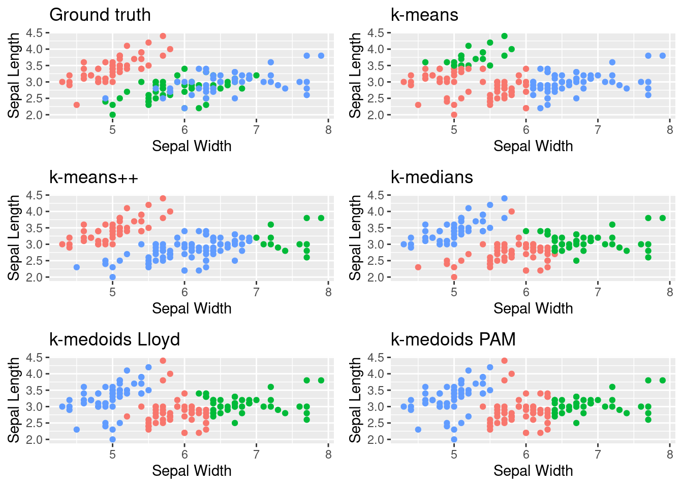
Let’s start by visualizing the results. Of course the colors for the “same” cluster can differ between the different algorithms, because they do not know which cluster belongs to which species.

set.seed(2)
df <- iris[, c("Sepal.Length", "Sepal.Width")]
species <- iris$Species
kmeans_clusters <- my_kmeans(df, k = 3, n_iter = 10, init = "random")
kmeanspp_clusters <- my_kmeans(df, k = 3, n_iter = 10, init = "kmeans++")
kmedians_clusters <- kmedians(df, k = 3, n_iter = 10)
kmedoids_lloyd_clusters <- kmedoids_lloyd(df, k = 3)

## [1] "Converged after 13 iterations."

kmedoids_pam_clusters <- kmedoids_pam(df, k = 3)

## [1] "Converged after 0 iterations."

# Helper function to create plots
plot_clusters <- function(df, cluster_id, title) {
  p <- ggplot(df, aes(Sepal.Length, Sepal.Width, color = factor(cluster_id))) + 
    geom_point(show.legend = FALSE) +
    labs(title = title,
         x = "Sepal Width", 
         y = "Sepal Length")
  return(p)
}

p_ground_truth <- plot_clusters(df, species, "Ground truth")
p_kmeans <- plot_clusters(df, kmeans_clusters, "k-means")
p_kmeanspp <- plot_clusters(df, kmeanspp_clusters, "k-means++")
p_kmedians <- plot_clusters(df, kmedians_clusters, "k-medians")
p_kmedoids_lloyd <- plot_clusters(df, kmedoids_lloyd_clusters$cluster_id, "k-medoids Lloyd")
p_kmedoids_pam <- plot_clusters(df, kmedoids_pam_clusters$cluster_id, "k-medoids PAM")

grid.arrange(p_ground_truth, p_kmeans, p_kmeanspp, p_kmedians, p_kmedoids_lloyd, p_kmedoids_pam, 
             ncol = 2)

Most algorithms do find more or less correct clusters, with the exception of k-medians. We also see that the PAM algorithm does actually not perform any swaps at all, highlighting the strength of its BUILD phase! Also keep in mind if you do compare the number of iterations between PAM and Lloyd k-medoids that PAM only performs a single swap per iteration, whereas the LLoyd k-medoids performs a swap for each current medoid, the number of total swaps is therefore k * iterations.

If you want to learn more about with which objective metrics you can judge your clustering outcomes, check out the corresponding section in my article on k-means.

Runtime

Finally, let’s compare the runtimes of the different algorithms, and let’s also check how much faster the implementation in FORTRAN from R is.

library(microbenchmark)
bench <- microbenchmark(
  base_kmeans = kmeans(df, centers = 3, iter.max = 10, algorithm = "Lloyd"),
  my_kmeans = my_kmeans(df, k = 3, n_iter = 10, init = "random"),
  my_kmeanspp = my_kmeans(df, k = 3, n_iter = 10, init = "kmeans++"),
  kmedians = kmedians(df, k = 3, n_iter = 10),
  kmedoids_lloyd = kmedoids_lloyd(df, k = 3),
  kmedoids_pam = kmedoids_pam(df, k = 3),
  times = 5
)

## Warning: did not converge in 10 iterations

## [1] "Converged after 13 iterations."

## Warning: did not converge in 10 iterations

## [1] "Converged after 5 iterations."
## [1] "Converged after 0 iterations."
## [1] "Converged after 0 iterations."
## [1] "Converged after 9 iterations."
## [1] "Converged after 0 iterations."
## [1] "Converged after 0 iterations."
## [1] "Converged after 3 iterations."
## [1] "Converged after 9 iterations."
## [1] "Converged after 0 iterations."

plot(bench)

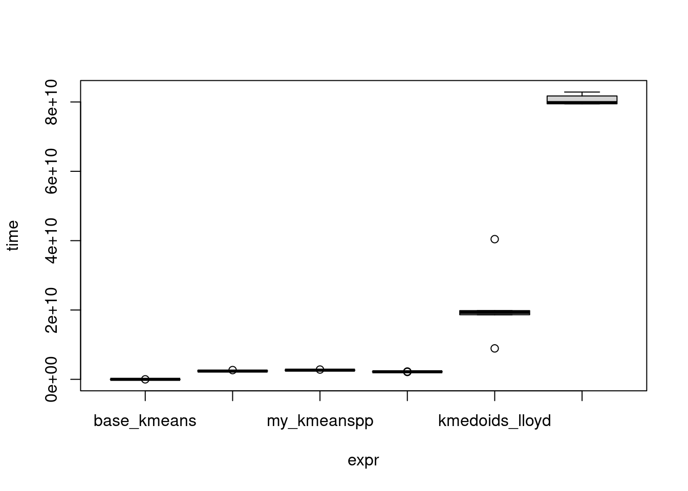
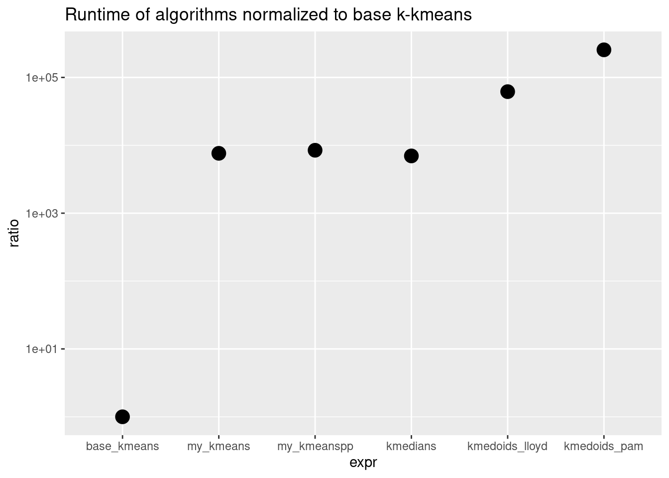
As expected, PAM is the slowest algorithm, followed by Lloyd style k-medoids. Since the other lines are very close on the scale lets look at ratios instead:

bench_df <- summary(bench)
bench_df$ratio <- bench_df$median / bench_df[bench_df$expr == "base_kmeans", "median"]

ggplot(bench_df, aes(x = expr, y = ratio)) +
  geom_count(show.legend = FALSE) + 
  scale_y_log10() + 
  labs(title = "Runtime of algorithms normalized to base k-kmeans",
       xlab = "Algorithm",
       ylab = "Ratio to base k-means")

Our vanilla k-means algorithm is 4000x slower than the base k-means! This demonstrates the drastic performance gain you can get if one implements an algorithm more efficiently and in a lower-level language, like C++. But our goal here was not efficiency, but understanding.

Summary

Congratulations if you made it this far. With PAM, you know now a very sophisticated clustering method that can be robustly applied to many data sets. Due to its high computational cost, it might not be completely suitable for very large data sets. If this is the case for you, check out algorithms designed for that, such as CLARA or CLARANS. This post also concludes my mini-series on k-means and related clustering algorithms. Stay tuned on what comes next!

Photo by Alina Grubnyak on Unsplash