How to cluster noisy data sets
The k-medians variation for robust outcomes
By Martin Helm in Data Science Machine Learning kmeans R
August 6, 2021
## Warning: package 'ggplot2' was built under R version 4.0.5
## Warning: package 'gridExtra' was built under R version 4.0.5
Introduction
If you have ever wanted to segment your data into groups, you have probably tried the famous k-means algorithm for it. Since it is so simple, it is widely used, but its simplicity also comes with several drawbacks. One of them is its sensitivity to outliers, as it uses classic euclidean distance as the dissimilarity metric. Unfortunately, real-world data sets often come with many outliers that you might not be able to remove completely during the data cleanup phase. If you have run into this problem, I want to introduce you to the k-medians algorithm. By using the median instead of the mean, and using a more robust dissimilarity metric, it is much less sensitive to outliers.
In this article, I will show you the following:
- k-medians intuition
- Implementation from scratch
k-medians intuition
k-medians tries to alleviate the sensitivity of k-means to outliers by choosing a different dissimilarity metric. Instead of the euclidean distance, we typically use the absolute difference, which is also called the L1 norm or the Manhattan or Taxicab distance (Because you can use it to calculate the number of turns a taxi needs to take to reach its target in a rectangular grid of blocks). This is much less sensitive to outliers because these are only contributing with their actual distance to the center, instead of the square of the distance, as is the case for euclidean distance:
$$ d(p,q) = \sum_{i = 1}^n |p_i - q_i| = ||.||^1 $$ with p and q being two n-dimensional vectors.
But one could also use other metrics here, if they are more appropriate, such as the Kullback-Leibler divergence to compare distributions.
To make it even more reliable, we also choose the median instead of the mean for the centers. So finally we need to optimize the following problem:
$$ argmin_C = \sum_{i = 1}^n \sum_{i \in C_i} |x - median(C_i) | $$ The approach of k-medians is very similar to k-means, it is again Llodyd’s algorithm. To summarize it briefly:
Input parameter k (number of clusters) and n_iter (number of iterations)
Randomly initialize k objects in the data set as centers
Do n_iter times:
  Assign each object to its closest center
  Calculate the new centers
You can find a much more detailed explanation on Lloyds algorithm in my post on k-means here.
Implementation from scratch in R
If we look at the programmatic implementation, we recognize that is it not as ubiquitously available as k-means. For example in R, there is no k-medians function available in the stats package. So let’s code it ourselves:
kmedians <- function(df, k, n_iter) {
  # define manhattan distance
  manhattan_distance <- function(x, y){
    return(sum(abs(x - y)))
  }

  # Initialize centers randomly
  centers <- df[sample(nrow(df), k), ]

  # Perform n_iter iterations
  for (iter in 1:n_iter) {
    # Calculate distances
    distances <- data.frame(matrix(NA, nrow = nrow(df), ncol = k))
    for (object_id in 1:nrow(df)) {
      for (center_id in 1:nrow(centers)) {
        # Use manhattan metric.
        distances[object_id, center_id] <- manhattan_distance(df[object_id, ], centers[center_id, ])
      }
    }

    # Assign each point to the closest center
    cluster_id <- apply(distances, 1, which.min)

    # Calculate new centers
    for (i in seq_len(k)) {
      this_cluster <- df[cluster_id == i,]
      # Calculate median instead of mean
      centers[k, ] <- apply(this_cluster, 2, median)
    }
  }
  return(cluster_id)
}
Testing it on the iris data set
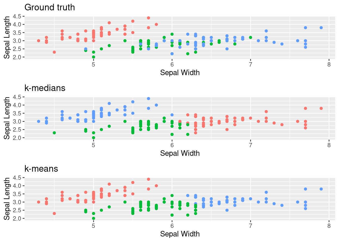
Next, let’s see how our function performs on the common iris data set. We will compare it also to the base R kmeans implementation, to see where they might differ:
set.seed(42)
df <- iris[, c("Sepal.Length", "Sepal.Width")]
species <- iris$Species
kmeans_clusters <- kmeans(x = df, centers = 3, iter.max = 10, nstart = 1)$cluster
kmedians_clusters <- kmedians(df, k = 3, n_iter = 10)

# Helper function to create plots
plot_clusters <- function(df, cluster_id, title) {
  p <- ggplot(df, aes(Sepal.Length, Sepal.Width, color = factor(cluster_id))) +
    geom_point(show.legend = FALSE) +
    labs(title = title,
         x = "Sepal Width",
         y = "Sepal Length")
  return(p)
}

p_ground_truth <- plot_clusters(df, species, "Ground truth")
p_kmeans <- plot_clusters(df, kmeans_clusters, "k-means")
p_kmedians <- plot_clusters(df, kmedians_clusters, "k-medians")
grid.arrange(p_ground_truth, p_kmedians, p_kmeans, ncol = 1)
 For this data set we only observe minor differences between k-medians and k-means,
but it also does not contain too many outliers to begin with.
Summary
As you can see, it is really similar to k-means, we really only use a different distance function and use the median.
One common misconception about k-medians is that the medians returned as centers always are actual points in the data set. This can be easily seen to not be true. Consider the following example cluster, consisting of 5 points for 2 dimensions:
kable(data.frame(observation = paste("point", 1:5), x = c(1, 2, 3, 4, 5), y = c(1, 2, 4, 3, 5)))
| observation | x | y |
|---|---|---|
| point 1 | 1 | 1 |
| point 2 | 2 | 2 |
| point 3 | 3 | 4 |
| point 4 | 4 | 3 |
| point 5 | 5 | 5 |
Because the median is calculated for each dimension separately in k-medians, the medians would be x = 3, and y = 3. But there exists no point (3, 3) in the data set.
Finally, of course you could couple k-medians together with an improved initialization, like kmeans++, to make it even more robust. You can find the details how to do that from my article on it. See you next time, when we will discuss probably the most advanced variation of k-means, partitioning around medoids, concluding this mini-series.