A deep dive into kmeans

Finally understand the most common clustering algorithm to its core

By Martin Helm in Data Science Machine Learning kmeans R pam

June 1, 2021

Introduction

Clustering problems are very common in data science. The underlying question is always to find groups of similar observations in your data. Depending on your domain, this might be customers with similar preferences, stocks that show similar performance or cells in your biological assay. The big appeal is that it is an unsupervised method. That means you do not need any labels beforehand, the algorithms instead finds the labels for you.

The simplest algorithm to do this is k-means, and I am sure you have already heard about it and probably used it. But I always find it helpful to code these algorithms from scratch, even the simple ones. Today’s post is structured as follows, simply jump to the section that interests you the most, or read everything for the complete picture:

Introduction to k-means theory
k-means implementation
Advantages and Disadvantages of k-means
How to find the ideal number of k
Relation to other clustering algorithms, like k-mediods or fuzzy-c-means
Summary

With that said, lets dive right into it.

K-means theory

Unsupervised learning methods try to find structure in your data, without requiring too much initial input from your side. That makes them very attractive for any kind of application. As with any other clustering algorithm, k-means wants to group observations together that are similar, while separating dissimilar points. K-means requires only 1 hyperparameter, which is k, the number of expected clusters. That makes it very easy to run, but also has some drawbacks, as discussed later. Mathematically, k-means focuses minimizing the within-cluster sum of squares (WCSS), which is also called the within-cluster variance, intracluster distance or inertia:

$$ WCSS_k = \sum_{x \in k} ||x - \bar{x} ||^2 $$

where k is the cluster and ||.||² is the euclidean norm, in this case the euclidean distance between two points.

Since we minimize over all clusters C, we can write the optimization function as follows:

$$ argmin_C = \sum_{i = 1}^k \sum_{x \in C_i} ||x - \bar{x} ||^2 = argmin_C \sum_{i = 1}^k |C_i| Var C_i $$

with $|C_i|$ being the cardinality of the cluster, i.e. the number of observations within it.

One can also interpret that as maximizing the total variance between clusters, also called the intercluster distance, as the law of total variance states:

$$\text{total Variance = explained variance (WCSS) + unexplained variance (intercluster distance)}$$

k-means implementation

We will walk through all steps of k-means, one at a time. For this implementation, I tried to be very explicit, to make the code as understandable as possible. Of course, this is not the fastest implementation, but the goal here is understanding first.

Since we will be using the iris data set in this example, let’s pretend for a minute that we are gardeners. We have worked hard to breed three different beautiful flowers, but unfortunately we forgot to add labels to our seedlings. They are not in bloom yet, but we really want to make sure to only plant the same flowers together. All we can do for now is measure the outer leafs, the so called sepals. Lets first have a look at the data (We will not need to load any packages in this example, as we really do it from scratch).

head(iris)

##   Sepal.Length Sepal.Width Petal.Length Petal.Width Species
## 1          5.1         3.5          1.4         0.2  setosa
## 2          4.9         3.0          1.4         0.2  setosa
## 3          4.7         3.2          1.3         0.2  setosa
## 4          4.6         3.1          1.5         0.2  setosa
## 5          5.0         3.6          1.4         0.2  setosa
## 6          5.4         3.9          1.7         0.4  setosa

As you can see, the data set contains information about the sepals, the petals and also from which of the three species the plant was, which is what we want to predict. So lets first select only the data we have in our example:

df <- iris[, c("Sepal.Length", "Sepal.Width")]
plot(df)

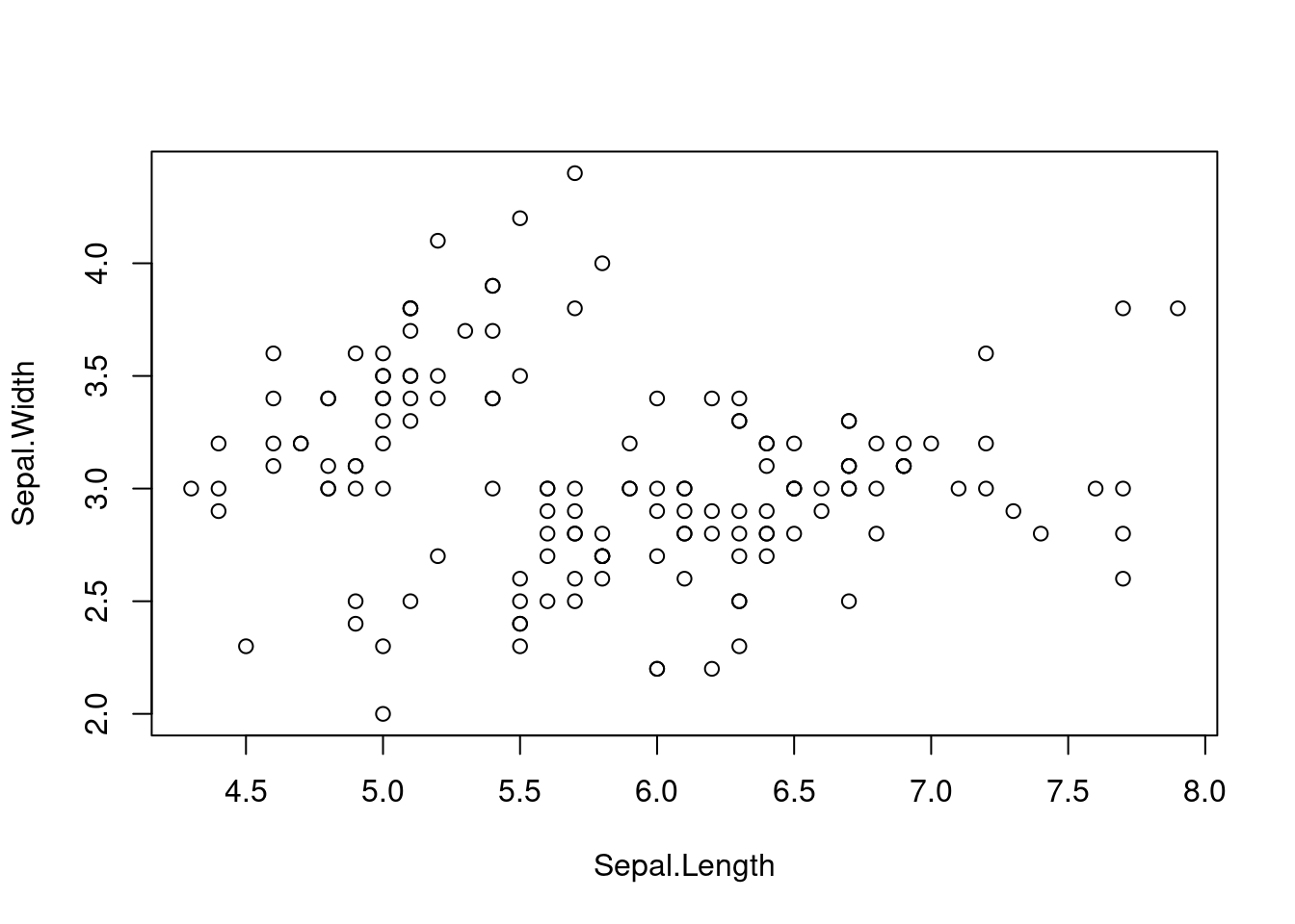
The visual inspection shows only two groups, although we expect 3 different species. So let’s see if k-means can find the third group as well.

Distance metric

First we need to define our distance metric - we will measure the distance of each point to a center with the euclidean distance:

euclidean_distance <- function(p1, p2) {
  dist <- sqrt( (p1[1] - p2[1])^2 + (p1[2] - p2[2])^2 )
  as.numeric(dist)
}

This distance function is of course only valid for the two-dimensional case, but one can easily expand that to any dimension you want. We wrap the output in a call to as.numeric() to remove any names, in case the input is a data.frame or a named vector.

Initialization

K-means requires an initial guess for the first centers. That also means, we need to input the number of expected centers to the algorithm, which is one of the most prominent drawbacks of k-means. We will cover this in its own section, for now lets assume we know that we had three different breeds.

To initialize the algorithm, we simply select three points at random from the dataset. To emphasize that we need to do this without replacement I wrote out this optional argument as well, even though the default is already set to FALSE.

k <- 3
centers <- df[sample(nrow(df), k, replace = FALSE), ]

Iteration

Next, we need to calculate the distance of each point to these centers.

distances <- matrix(Inf, nrow = nrow(df), ncol = k)
for (i in seq_len(nrow(df))) {
  for (j in seq_len(k)) {
    distances[i, j] <- euclidean_distance(df[i, ], centers[j, ])
  }
}

Now we can assign each point to it’s closest center. To do that we go over the results by row (MARGIN = 1) and select the entry with the lowest distance.

cluster_id <- apply(distances, 1, which.min)

Finally, we need to calculate the new centers for each cluster. To stay true to the highly explicit coding style we also do this in a for loop.

# Calculate new centers
for (i in seq_len(k)) {
  this_cluster <- df[cluster_id == i,]
  centers[k, ] <- apply(this_cluster, 2, mean)
}

And voilá, that’s all there is to one round of k-means. Since we effectively move the coordinates of the center during this step, k-means belong the group of coordinate-descent algorithms.

But of course, one iteration is not sufficient. Instead we need to iterate multiple times over the data set and always adjust our centers. In our implementation we choose to run k-means a defined number of iterations before we terminate. To do that, we can wrap everything in a while loop and put it in a function. Alternatively, one could include a check to terminate early if the algorithm has converged (i.e. the centers do not change between two iterations), or the change in the total WCSS is below a defined threshold.

my_kmeans <- function(data, k, n_iterations) {
  # Helper function for euclidean distance 
  euclidean_distance <- function(p1, p2) {
    dist <- sqrt(sum((p1-p2)^2))
    return(dist)
  }
  # Initialize centers randomly
  centers <- df[sample(nrow(df), k, replace = FALSE), ]
  
  # Perform n iterations
  iteration <- 1
  while(iteration < n_iterations) {
    # Calculate distance of each point to each center
    distances <- matrix(Inf, nrow = nrow(df), ncol = k)
    for (i in seq_len(nrow(df))) {
      for (j in seq_len(k)) {
        distances[i, j] <- euclidean_distance(df[i, ], centers[j, ])
      }
    }
    
    # Assign each point to the closest center
    cluster_id <- apply(distances, 1, which.min)
    
    # Calculate new centers
    for (i in seq_len(k)) {
      this_cluster <- df[cluster_id == i,]
      centers[k, ] <- colMeans(this_cluster)
    }
    
    iteration <- iteration + 1
  }
  
  cluster_id
}

Analysis of our test data

Let’s run our analysis and compare it to the real species

set.seed(42)
cluster_id <- my_kmeans(data = df, k = 3, n_iterations = 10)

par(mfrow = c(1,2))
plot(df, col = cluster_id, main = "K-means result")
plot(df, col = iris$Species, main = "Ground-truth species")

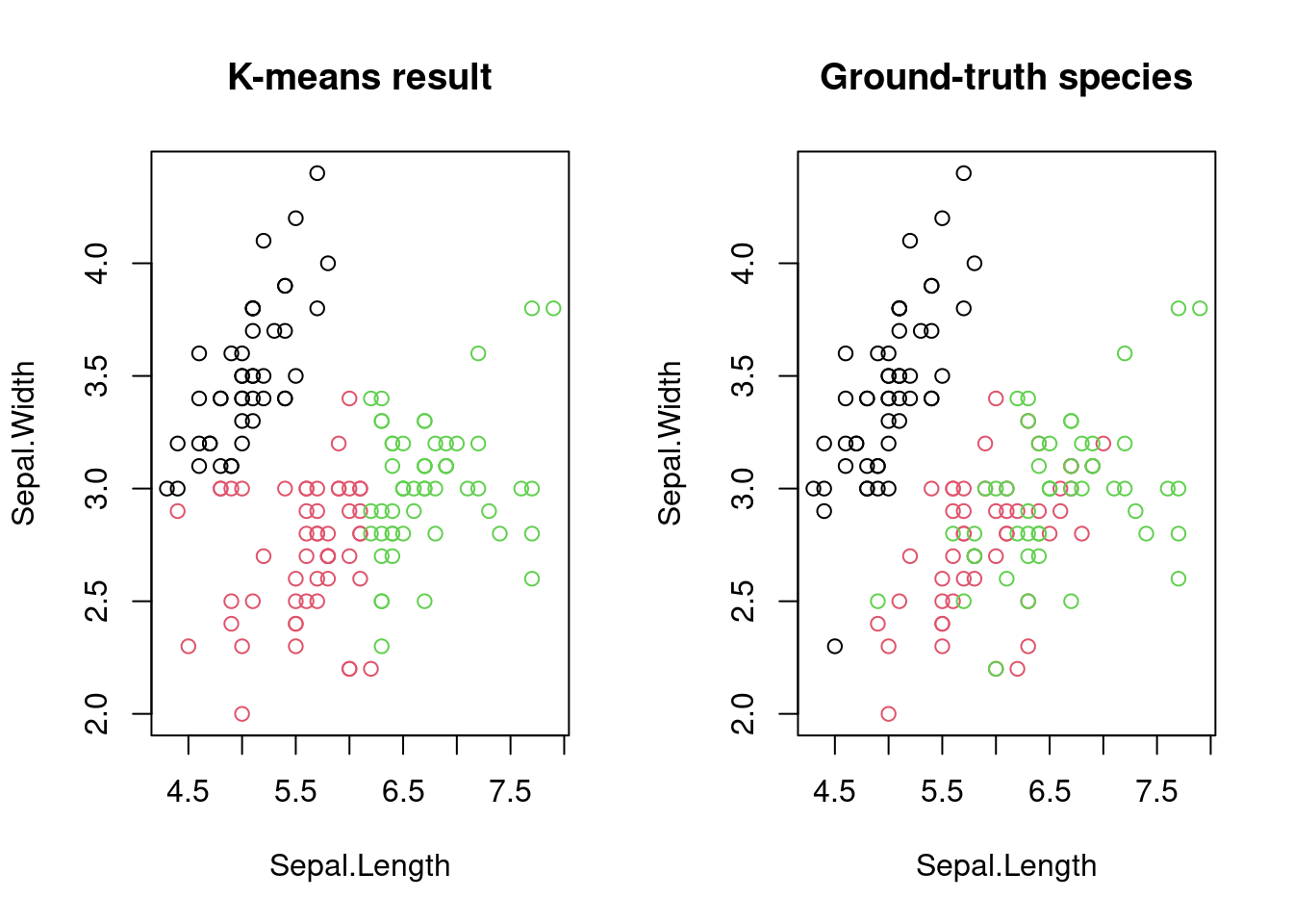
As you can see, K-means was indeed able to separate the plants into three groups, which are similar to the underlying ground-truth.

How to find the ideal number of k

As we have seen, k-means requires us to input the expected number of clusters. This is a serious limitations, as we might not necessarily know this in advance. Moreover, k-means will always output a clustering with the specified number of k clusters, no matter whether this makes sense or not. So how can we deal with this? There are several approaches possible.

Elbow method

One very common solution is the so called elbow method. We perform k-means with several candidate values of k and then select the best one. To do this selection we use the total WCSS, i.e. the sum of the WCSS over all clusters.

To explain this a bit more intuitively, imagine first an example with k = 1. All events will belong to the same cluster, that means the total WCSS will be equal to to the total sum of squares in the dataset. If we increase k to 2, at least some points will belong to the second cluster. This will decrease the SS within the first cluster, and and also the total WCSS will be smaller as the total WCSS with k = 1. So the higher k becomes, the smaller the WCSS will be. In the extreme case of k = number of observations, the WCSS will be 0.

To select the best k, we need to find the best tradeoff between this reduction in the WCSS and overfitting of our model to the data. The elbow method does that by selecting the point with the strongest “bend” in this behavior of the WCSS. To illustrate that, lets plot the behavior in our data for values of k from 1 to 10. We will use the already implemented kmeans method from now on, as it is faster and has the WCSS already implemented, which is the tot.withinss element of the result list.

within_cluster_ss <- c()
for (k in 1:10) {
  within_cluster_ss[k] <- kmeans(df, k)$tot.withinss
}
plot(1:10, within_cluster_ss, xlab = "Number of clusters", ylab = "Total within-cluster distances", type = "b")

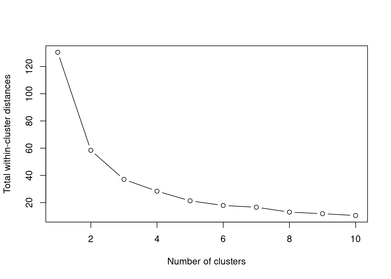
We can speculate that the point with the strongest bend is at k = 3, but it might as well be at k = 4.

In addition, it would also be great to get this selection automatically, without the need for us to manually select it. We can automate this with a small helper function. First we fit a line between the maximum and the minimum point. Then we calculate the distance between each point to this line. The point with the highest distance is the elbow point. Alternatively, one could calculate the point with the maximum absolute second derivative.

find_elbow <- function(x, y) {
  max_x_x <- max(x)
  max_x_y <- y[which.max(x)]
  max_y_y <- max(y)
  max_y_x <- x[which.max(y)]
  
  max_df <- data.frame(x = c(max_y_x, max_x_x), 
                       y = c(max_y_y, max_x_y))
  
  line_fit <- lm(max_df$y ~ max_df$x)
  
  df <- data.frame(x = x, y = y)
  
  distances <- apply(df, 1, function(this_point) {
    abs(coef(line_fit)[2]*this_point[1] - this_point[2] + coef(line_fit)[1]) / sqrt(coef(line_fit)[2]^2 + 1^2)
  })
  
  elbow <- c(x = x[which.max(distances)],
             y = y[which.max(distances)])
  
  elbow
}

elbow <- find_elbow(x = 1:10, y = within_cluster_ss)
elbow

##       x       y 
##  3.0000 37.0507

Indeed it returns k = 3, but this is only a heuristic. For example, rerun the same example, but this time vary k between 1 and 20. You will see that in this case it will return k = 4 as the best number of clusters.

Silhouette score

Another method to assess which k fits the data best is the so-called silhouette score. It measures the similarity of points within a cluster and compares it to the similarity of the points to the other clusters. It ranges between -1 and 1 ,with -1 indicating points that are very dissimilar to their assigned clusters, while 1 indicates points that are highly similar to their cluster. A value of 0 indicates that this point lies at the edge between two neighboring clusters. Let’s go through it step-by-step:

After running k-means, for each cluster we calculate the average distance of each point to all other points within the same cluster. One can also interpret that as a how similar each point is to the cluster it was assigned to, with a low value showing a high similarity. Let $i$ be a data point in the cluster $C_i$ , and $d$ the distance metric (in our case the euclidean distance). Then the distance for this point i to its cluster is defined as: $$ \text{distance assigned cluster(i)} = \frac{1}{|C_i|} \sum_{j \in C_i} d(i,j) $$

With $|C_i|$ again being the cardinality of the cluster, i.e. the number of elements in it. A small value indicates a point that is very similar to its cluster.

Alternatively, we can exclude the distance of a point to itself, which yields: $$ \text{distance assigned cluster(i)} = \frac{1}{|C_i| - 1} \sum_{j \in C_i, i \ne j} d(i,j) $$

In the second step, we calculate the similarity of this point to the other clusters. So for each other cluster, we calculate the average distance of point $i$ to all points $j$ belonging to cluster $k$. The dissimilarity is then defined as the average distance to the closest cluster, which is also called the “neighboring cluster” for point $i$.

$$ \text{distance neighbor cluster (i)} = min_{k \ne i} \frac{1}{|C_k|} \sum{j \in C_k} d(i,j) $$

Finally, we need to weigh this to each other, which yields the silhouette score:

$$ s(i) = \frac{\text{distance neighbor cluster(i) - distance assigned cluster(i)}}{max(\text{distance neighbor cluster(i), distance assigned cluster(i)})} $$

Let’s assume we have a point at the very center of its assigned cluster. In that case, the distance to its assigned cluster is 0, which yields $$ s(i) = \frac{\text{distance neighbor cluster}}{\text{distance neighbor cluster}} = 1 $$

On the contrary, a point at the boundary between two clusters will have equal distances to the center of its assigned cluster and the center of the nearest neighboring cluster. It follows: $$ s(i) = \frac{0}{max(\text{distance neighbor cluster(i), distance assigned cluster(i)})} = 0 $$

In theory, the silhouette score can also become negative (until -1), which indicates a point that should have been assigned to a different cluster. For k-means that should not happen, because we assign the points based on the distance.

silhouette <- function(data, cluster_id) {
  silhouette <- c()
  clusters <- unique(cluster_id)
  for (cluster in clusters) {
    this_cluster <- data[cluster_id == cluster, ]
    distances <- as.matrix(dist(this_cluster)) # calculate euclidean distances
    distance_assigned_cluster <- (1 / (nrow(this_cluster) - 1)) * colSums(distances)
    
    distance_neighbor_cluster <- c()
    other_clusters <- clusters[clusters != cluster]
    for (i in seq_len(nrow(this_cluster))) {
      distance_other_clusters <- c()
      for (j in other_clusters) {
        other_cluster <- data[cluster_id == j, ]
        data_tmp <- rbind(this_cluster[i, ], other_cluster)
        distances <- as.matrix(dist(data_tmp))
        distances <- distances[-1, 1]
        distance_other_cluster <- mean(distances)
        distance_other_clusters <- c(distance_other_clusters, distance_other_cluster)
      }
      distance_neighbor_cluster[i] <- min(distance_other_clusters)
    }
    
    # We take advantage of the pmax function in the denominator, which gives the
    # "parallel" or pairwise maxima between two vectors.
    silhouettes_this_cluster <- (distance_neighbor_cluster - distance_assigned_cluster) / pmax(distance_neighbor_cluster, distance_assigned_cluster)
    silhouette <- c(silhouette, silhouettes_this_cluster)
  }
  silhouette
}

For cases where a cluster only contains one single member, we need to define a fixed score. We choose 0, as it is a neutral choice between in the silhouette range of -1 to 1. So in the case of $$ s(i) = 0, if|C_i| = 1 $$

For programmatic assessment whether the clustering is good, one typically then calculates the mean $\bar{s}$ over all points for each $k$. We then choose the $k$ with the highest value of $\bar{s}$.

silhouette_scores <- c()

for (k in 2:10) {
  cluster_id <- kmeans(df, k)$cluster
  silhouettes <- silhouette(df, cluster_id)
  silhouette_scores <- cbind(silhouette_scores, silhouettes)
}

colnames(silhouette_scores) <- 2:10
silhouette_scores <- apply(silhouette_scores, 2, mean)
best_k <- names(which.max(silhouette_scores))
best_k

## [1] "2"

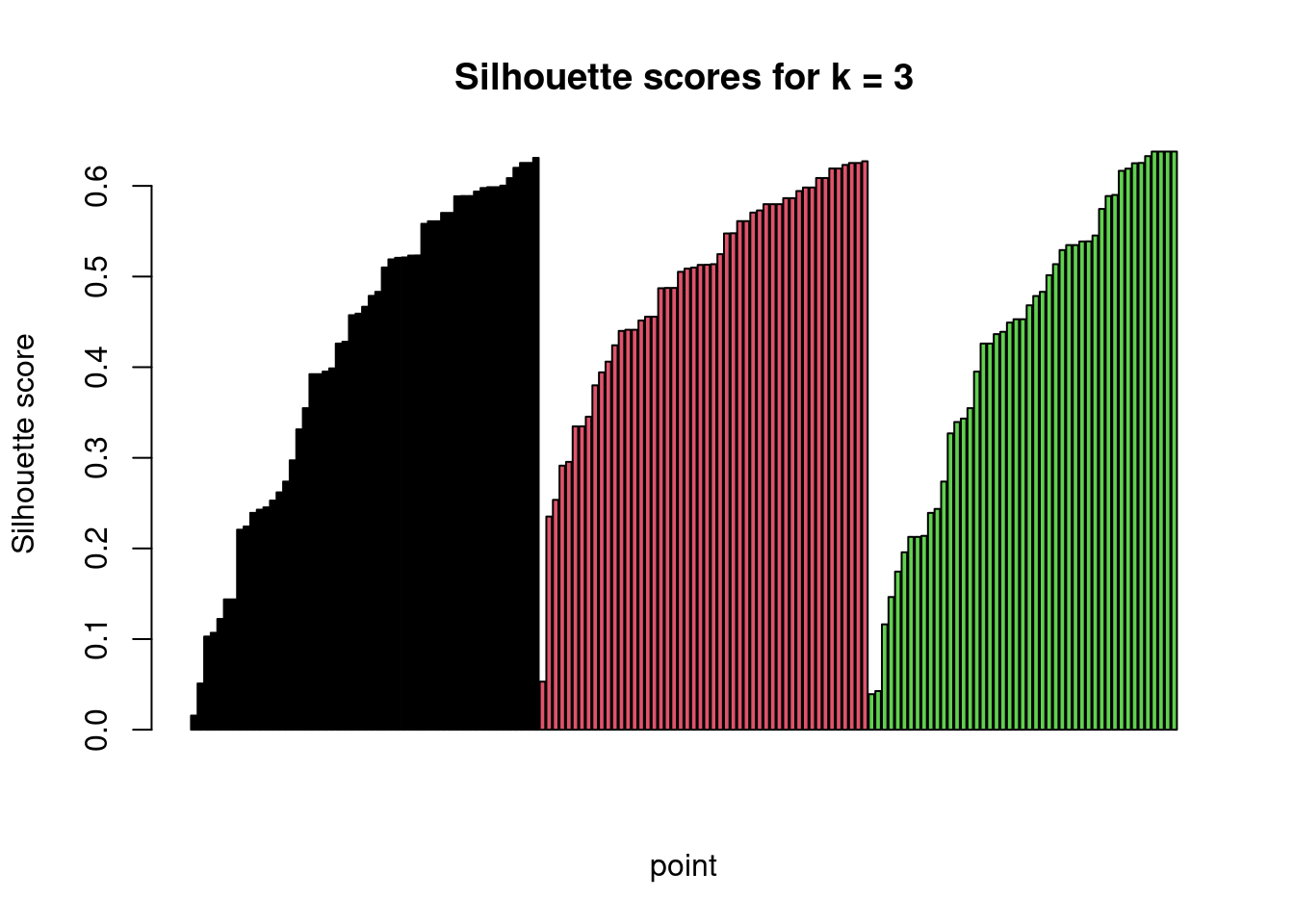
Alternatively, one can plot all $s(i)$ values for a given $k$ and assess the clustering visually:

k <- 3
kmeans_res <- kmeans(df, k)
cluster_id <- kmeans_res$cluster
silhouettes <- silhouette(df, cluster_id)
result_df <- data.frame(cluster_id = cluster_id, silhouette = silhouettes)
result_df <- result_df[order(result_df$cluster_id, result_df$silhouette), ]
barplot(result_df$silhouette, col = result_df$cluster_id, 
        main = "Silhouette scores for k = 3", xlab = "point", 
        ylab = "Silhouette score")

Assessment of clustering result

After you have settled on the best $k$ and done your analysis, there are still some steps do be done. First of all, you should assess the quality of your clustering.

Cluster cardinality

We already learned that cluster cardinality is the number of events in a cluster. Depending on your knowledge of the data, you might expect equally sized clusters, or maybe also different sized clusters.

cluster_cardinality <- table(cluster_id)
barplot(cluster_cardinality, main = "Cluster Cardinality", xlab = "cluster id", 
        ylab = "Number of points in cluster", col = c("firebrick2", "orange", "chartreuse4"))

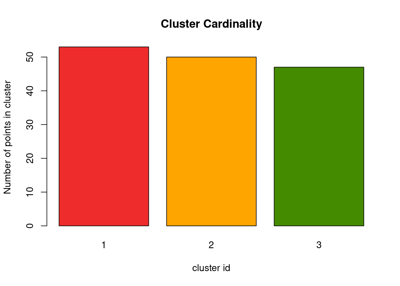
I have seen several people suggest that clusters should always be equal in size, but I don’t think that is true. What if there are really more rare populations in the data that indeed are forming their own group? That might be true for patients with rare characteristics, social network analysis, cells with a unique gene expression level or simply differences during manufacturing of a good you are investigating. So don’t get too worried if your clusters show differing cardinality, but look into the outliers nonetheless.

Cluster cardinality vs cluster magnitude

Cluster magnitude describes the total distances of all points in a cluster to its center. Luckily, the k-means implementation in R already computes these values for you:

cluster_magnitude <- kmeans_res$withinss
barplot(cluster_magnitude, main = "Cluster Magnitude", xlab = "cluster id",
        ylab = "Total distances within cluster", names.arg = 1:3, 
        col = c("firebrick2", "orange", "chartreuse4"))

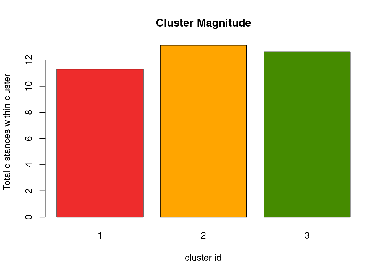
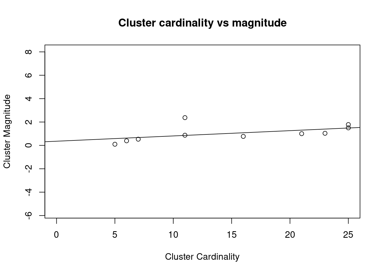
This value alone doesn’t enable much insight, similar to the cluster cardinality alone. But combing both of them will show better trends in the result. Intuitively one would expect that clusters with few members (i.e. low cardinality) also have a low total differences of these points to the cluster center. So both values should positively correlate with each other. If this is not the case this would suggest a disperse cluster, which could mean that these are actually noise points.

plot(x = as.numeric(cluster_cardinality), y = cluster_magnitude,
     asp = 1, xlim = c(0, max(cluster_cardinality)), ylim = c(0, max(cluster_magnitude)),
     main = "Cluster cardinality vs magnitude",
     xlab = "Cluster Cardinality", ylab = "Cluster Magnitude", 
     col =  c("firebrick2", "orange", "chartreuse4"))

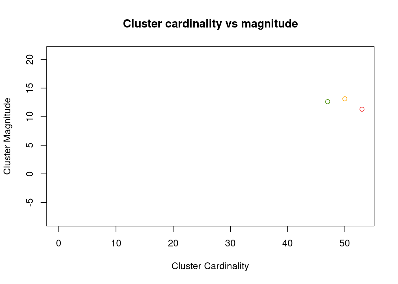
As we can see, this plot is not too helpful for low values of k. To still bring the point across, let’s plot the result of k = 10.

kmeans_10 <- kmeans(df, 10)
cluster_cardinality_10 <- table(kmeans_10$cluster)
cluster_magnitude_10 <- kmeans_10$withinss
plot(x = as.numeric(cluster_cardinality_10), y = cluster_magnitude_10,
     asp = 1, xlim = c(0, max(cluster_cardinality_10)), ylim = c(0, max(cluster_magnitude_10)),
     main = "Cluster cardinality vs magnitude",
     xlab = "Cluster Cardinality", ylab = "Cluster Magnitude")
lm <- lm(cluster_magnitude_10 ~ cluster_cardinality_10)
abline(a = lm$coefficients[1], b = lm$coefficients[2])

Cluster characteristics

Finally, the last but probably most important step is to describe your clusters. Depending on what domain you are in, that might be simple summary statistics of the dimensions (in our example, how long/wide are the petals), or other descriptions such as image intensity, gene expression levels and so on. After all, when running a cluster analysis you are interested in what groups are present, so describe them in detail after you found them!

Advantages of k-means

After this deep dive into the implementation, lets focus on a few more high-levels characteristics of k-means. Its a popular algorithms and comes with several advantages:

It is easy to understand conceptionally

As we have seen, the theory is straightforward and one can easily visualize and understand the concept behind k-means.

It is implemented in basically all programming languages

Virtually every common programming language comes with an implementation of k-means, which makes it easy to run it on a data set.

It has only 1 hyperparameter

k, the number of clusters

It scales well to the number of observations.

Its complexity is O(nkdi), where

n = the number of d-dimensional vectors

k = the number of clusters

i = the number of iterations until convergence

Disadvantages of k-means

On the other hand, thesimplicity of k-means also brings some major disadvantages:

It requires prior knowledge of k

This is a major drawback, as often one doesn’t know the number of clusters that are present in the data. Also, it will always return exactly $k$ numbers of clusters, no matter how many might actually make sense in the data. We can alleviate this a bit by trying different $k$ and choosing the best one, but as we have seen, this also does not work always.

It is a heuristic algorithm

As the actual problem is NP-hard to solve, usually a heuristic is used to find a solution, mostly Loyd’s algorithm. That means that the result one gets returned could also be only a local optimum.

It is not deterministic

Since the initialization is random and we use a heuristic, multiple runs of k-means can return vastly different results.

It is heavily influenced by outliers

As the euclidean distance is the square of the difference between two points, outliers heavily influence the outcome.

It scales poorly to increasing dimensions

With increase numbers of dimensions, the euclidean distance between them becomes very similar. This is known as the curse of dimensionality. But if the distance is not meaningful anymore, our algorithm also falls apart.

Assumptions made by k-means

As with any algorithm, there are a few assumptions that are made, either explicitly or implicitly

Clusters are spherical/The variance to a center point is meaninfull

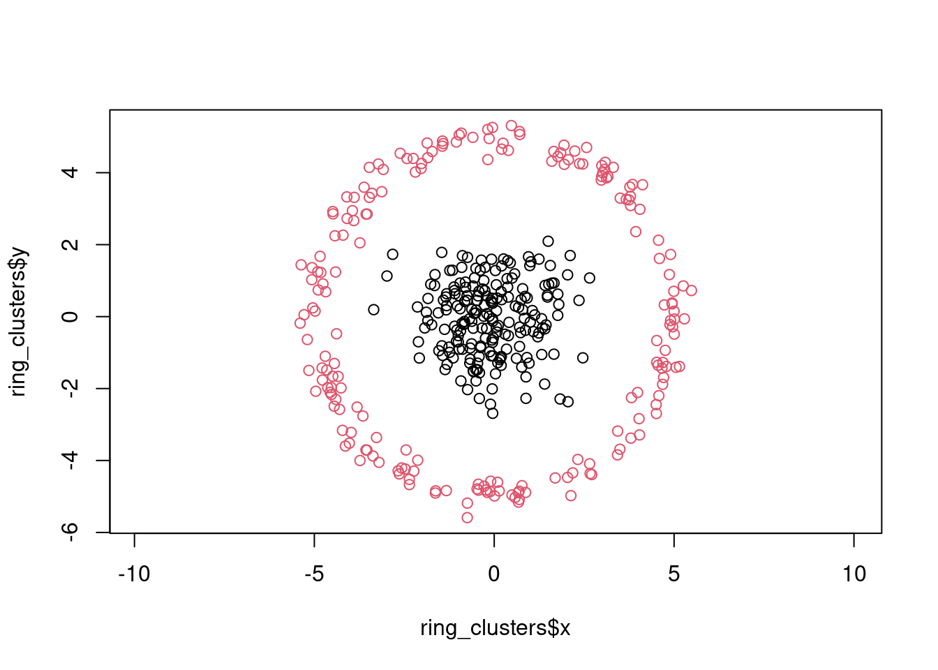
As the distance metric is symmetric, it will always find clusters with a spherical border. Note that this does not mean that it works well for all point clouds that have a circular shape, for example consider a ring shaped cluster:

inner_cluster <- data.frame(x = rnorm(200), y = rnorm(200), cluster = 1)
outer_cluster <- data.frame(r = rnorm(200, 5, .25), 
                            theta = runif(200, 0, 2 * pi),
                            cluster = 2)
outer_cluster$x <- outer_cluster$r * cos(outer_cluster$theta)
outer_cluster$y <- outer_cluster$r * sin(outer_cluster$theta)
outer_cluster <- outer_cluster[, c("x", "y", "cluster")]
ring_clusters <- rbind(inner_cluster, outer_cluster)
plot(ring_clusters$x, ring_clusters$y, col = ring_clusters$cluster, asp = 1)

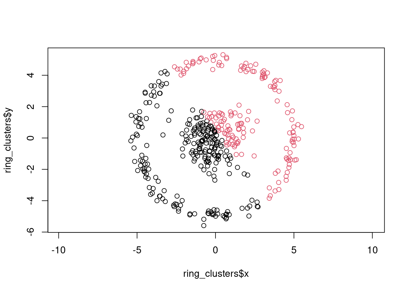
k-means will not be able to separate the inner point cloud from the outer ring:

cluster_id <- kmeans(ring_clusters[, c("x", "y")], centers = 2)$cluster
plot(ring_clusters$x, ring_clusters$y, col = cluster_id, asp = 1)

Clusters are equally sized

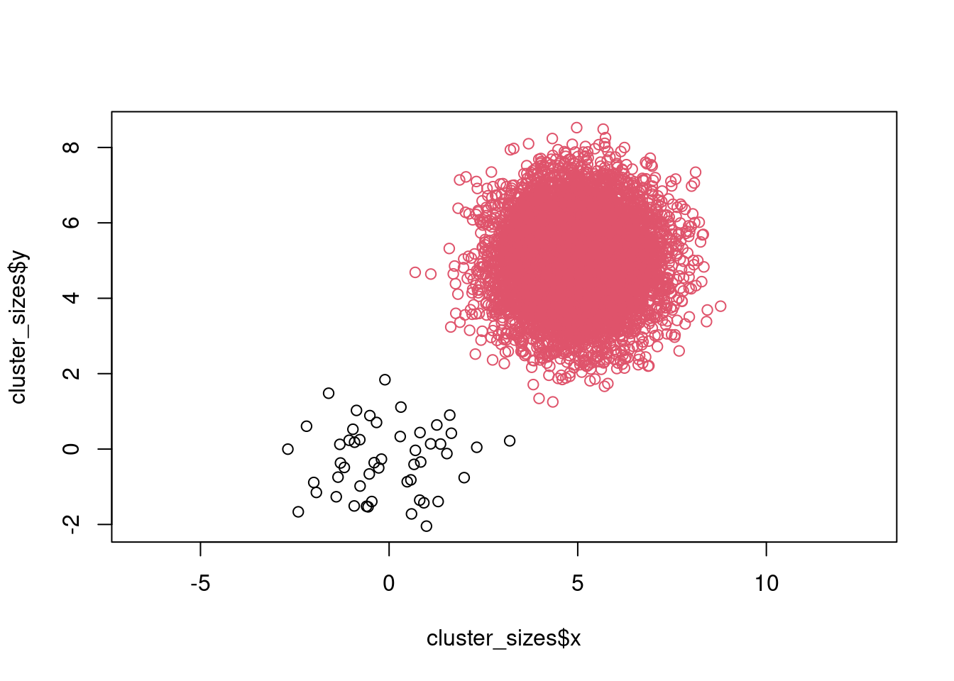
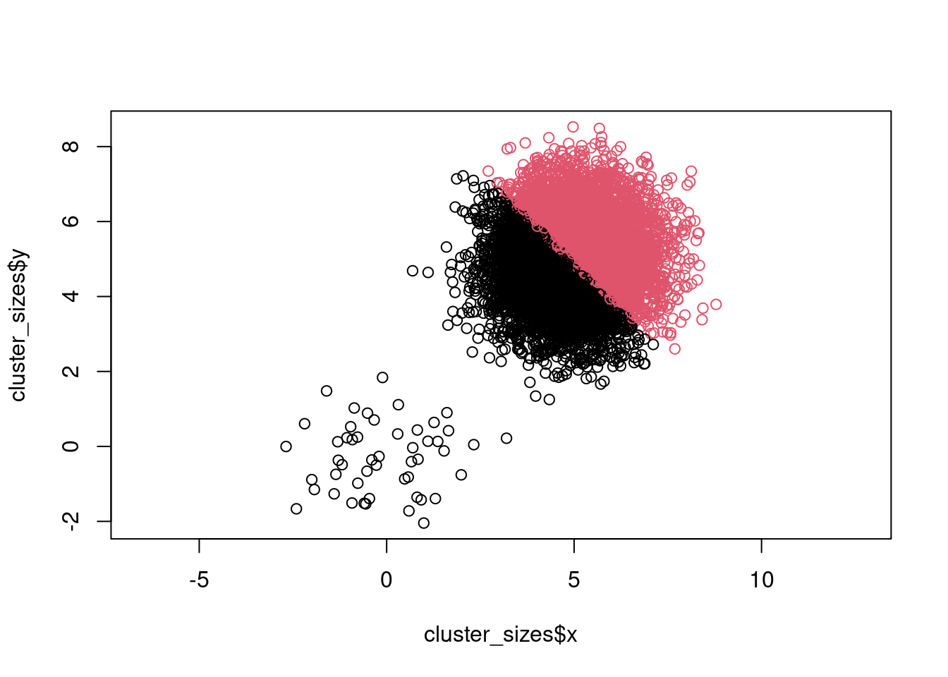
There are several posts and threads on stack overflow discussing, whether k-means makes the assumption that clusters should be equally sized. The underlying metric does not make that assumption explicitly, but one can see that it makes sense from how the algorithm work. Suppose we have 2 very differently sized clusters. Since we choose the initial centers randomly, we have a high probability that the are both initialized in the large cluster. The small cluster will be unable to “attract” one of the centers, resulting in wrong result. To see that in action, lets construct 2 clusters with sizes 10 and 1000.

cluster_small <- data.frame(x = rnorm(50), y = rnorm(50), cluster = 1)
cluster_large <- data.frame(x = rnorm(10000) + 5, y = rnorm(10000) + 5, cluster = 2)
cluster_sizes <- rbind(cluster_small, cluster_large)
plot(cluster_sizes$x, cluster_sizes$y, col = cluster_sizes$cluster, asp = 1)

Now lets see what happens when we run k-means:

cluster_id <- kmeans(cluster_sizes[, c("x", "y")], centers = 2)$cluster
plot(cluster_sizes$x, cluster_sizes$y, col = cluster_id, asp = 1)

Dimensions are equally important

This goes in the same direction as the assumption that clusters are roughly spherical. If one dimension has a much larger scale than the others, it will dominate the clustering. Therefore it is very important to normalize your data before clustering.

Relation to other clustering methods

k-means++

k-means++ uses an improved initialization. Instead of randomly selecting all initial centers, it chooses only the first center randomly. All following centers are then chosen in a way that they have the maximum distance between the new center and all already existing centers.

k-medians

k-medians chooses the median instead of the mean for the cluster center computation. Typically it uses the Manhatten distance instead of the Euclidean distance as its metric, but also more complex metrics such as Kullback-Leibler divergence can be used.

k-mediods/PAM/k-center

k-mediods chooses the most representative point of the cluster as the center, so the center is always an actual data point in your data set. This is not to be confused with k-medians, where the center does not need to be an actual data point. This can be seen because the medians in two dimensions might not come from the same point!

It also uses a slightly different iterative step: After initialization, for each cluster it tries each of its containing points as a potential new cluster center and picks the one that minimizes the chosen dissimilarity metric.

Finally, it is also very flexible in the dissimilarity metric one wants to use.

fuzzy-c-means

Instead of hard clustering, it assigns a probability of each point to belong to a given cluster. This means a point can be a member of multiple clusters, which might make sense in some cases (for example genes belonging to multiple pathways).

Gaussian mixture models

One can also interpret k-means as a hard clustering variant of a gaussian mixture model that does not consider covariances. The expectation step is the where each observation is assigned to its closest center. The maximization step is where the centers are recomputed.

Summary

To conclude, we have seen that k-means is a simple and intuitive algorithm that can be quickly applied in basically any programming language to a data set. Its main drawback is the required input of the expected number of clusters. Still, its abundance and simplicity make it a useful tool to quickly run it on your data to familiarize yourself with it.

Photo by Evie S. on Unsplash